Table of Contents
Support Vector Machine or SVM is one of the most popular Supervised Learning algorithms, which is used for Classification as well as Regression problems. However, primarily, it is used for Classification problems in Machine Learning.
The goal of the SVM algorithm is to create the best line or decision boundary that can segregate n-dimensional space into classes so that we can easily put the new data point in the correct category in the future. This best decision boundary is called a hyperplane.
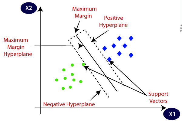
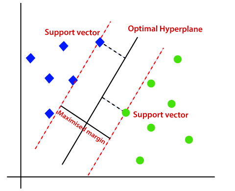
SVM chooses the extreme points/vectors that help in creating the hyperplane. These extreme cases are called as support vectors, and hence the algorithm is termed as Support Vector Machine. Consider the below diagram in which there are two different categories that are classified using a hyperplane:
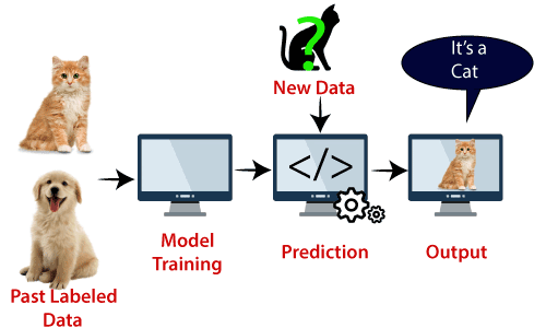
Example: SVM can be understood with the example that we have used in the KNN classifier. Suppose we see a strange cat that also has some features of dogs, so if we want a model that can accurately identify whether it is a cat or dog, so such a model can be created by using the SVM algorithm. We will first train our model with lots of images of cats and dogs so that it can learn about different features of cats and dogs, and then we test it with this strange creature. So as support vector creates a decision boundary between these two data (cat and dog) and choose extreme cases (support vectors), it will see the extreme case of cat and dog. On the basis of the support vectors, it will classify it as a cat. Consider the below diagram:
SVM algorithm can be used for Face detection, image classification, text categorization, etc.
Enroll in our certificate program in data science and Machine learning
Types of SVM
SVM can be of two types:
- Linear SVM: Linear SVM is used for linearly separable data, which means if a dataset can be classified into two classes by using a single straight line, then such data is termed as linearly separable data, and classifier is used called as Linear SVM classifier.
- Non-linear SVM: Non-Linear SVM is used for non-linearly separated data, which means if a dataset cannot be classified by using a straight line, then such data is termed as non-linear data and classifier used is called as Non-linear SVM classifier.
Hyperplane and Support Vectors in the SVM algorithm:
1: Which of the following algorithms is most suitable for classification tasks?
Hyperplane in SVM: There can be multiple lines/decision boundaries to segregate the classes in n-dimensional space, but we need to find out the best decision boundary that helps to classify the data points. This best boundary is known as the hyperplane of SVM.
The dimensions of the hyperplane depend on the features present in the dataset, which means if there are 2 features (as shown in image), then hyperplane will be a straight line. And if there are 3 features, then hyperplane will be a 2-dimension plane.
We always create a hyperplane that has a maximum margin, which means the maximum distance between the data points.
Support Vectors:
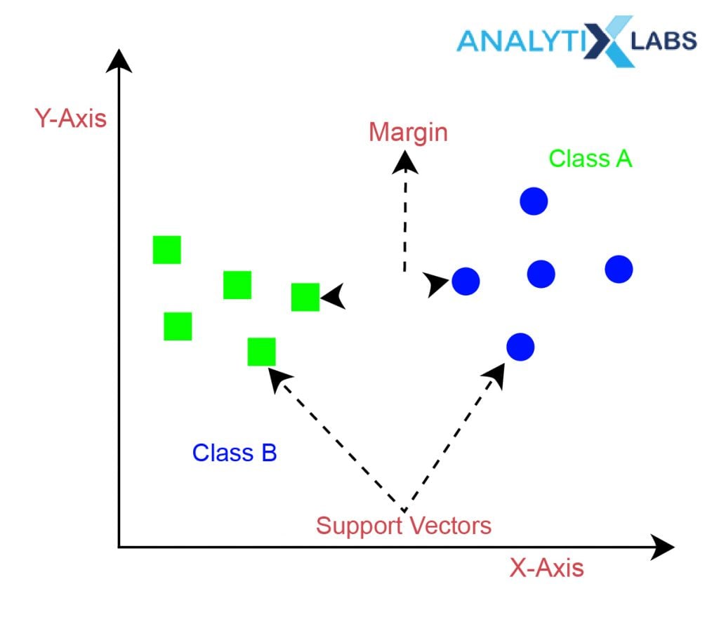
The data points or vectors that are the closest to the hyperplane and which affect the position of the hyperplane are termed as Support Vector. Since these vectors support the hyperplane, hence it is called as a Support vector.
 Start Coding Today! Enroll Now with Easy EMI Options.

Equip yourself with in-demand skills to land top-tier roles in the data-driven world.
Start Learning Now with EMI OptionsSVM Algorithm Steps
If the functioning of SVM classifier is to be understood mathematically then it can be understood in the following ways-
Step 1: SVM algorithm predicts the classes. One of the classes is identified as 1 while the other is identified as -1.
Step 2: As all machine learning algorithms convert the business problem into a mathematical equation involving unknowns. These unknowns are then found by converting the problem into an optimization problem. As optimization problems always aim at maximizing or minimizing something while looking and tweaking for the unknowns, in the case of the SVM classifier, a loss function known as the hinge loss function is used and tweaked to find the maximum margin.
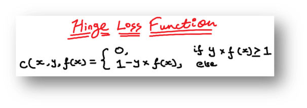
Step 3: For ease of understanding, this loss function can also be called a cost function whose cost is 0 when no class is incorrectly predicted. However, if this is not the case, then error/loss is calculated. The problem with the current scenario is that there is a trade-off between maximizing margin and the loss generated if the margin is maximized to a very large extent. To bring these concepts in theory, a regularization parameter is added.
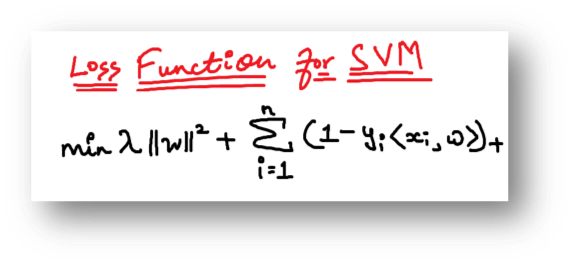
Step 4: As is the case with most optimization problems, weights are optimized by calculating the gradients using advanced mathematical concepts of calculus viz. partial derivatives.
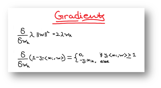
Step 5: The gradients are updated only by using the regularization parameter when there is no error in the classification while the loss function is also used when misclassification happens.
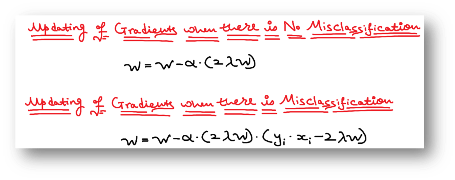
Step 6: The gradients are updated only by using the regularization parameter when there is no error in the classification, while the loss function is also used when misclassification happens.
Experience the power of our machine learning course with a free demo – Enroll Now!
How does SVM works?
Linear SVM:
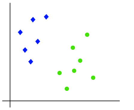
The working of the SVM algorithm can be understood by using an example. Suppose we have a dataset that has two tags (green and blue), and the dataset has two features x1 and x2. We want a classifier that can classify the pair(x1, x2) of coordinates in either green or blue. Consider the below image:
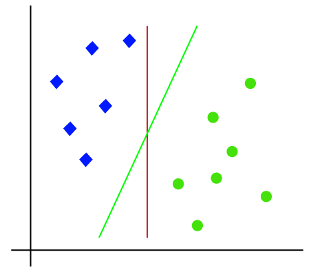
So as it is 2-d space so by just using a straight line, we can easily separate these two classes. But there can be multiple lines that can separate these classes. Consider the below image:
Hence, the SVM algorithm helps to find the best line or decision boundary; this best boundary or region is called as a hyperplane. SVM algorithm finds the closest point of the lines from both the classes. These points are called support vectors. The distance between the vectors and the hyperplane is called as margin. And the goal of SVM is to maximize this margin. The hyperplane with maximum margin is called the optimal hyperplane.
Non-Linear SVM:
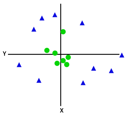
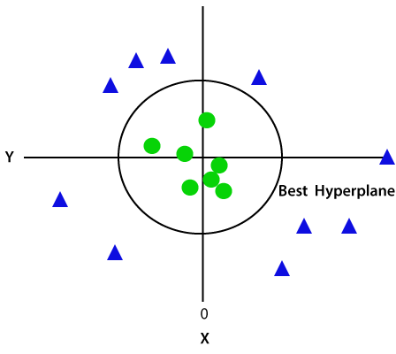
If data is linearly arranged, then we can separate it by using a straight line, but for non-linear data, we cannot draw a single straight line. Consider the below image:
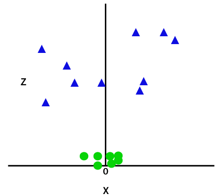
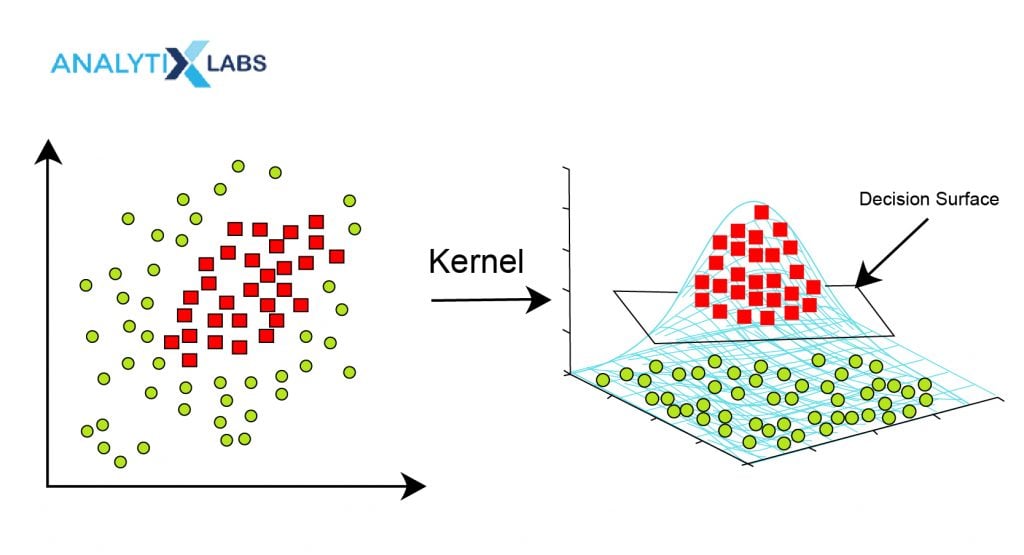
So to separate these data points, we need to add one more dimension. For linear data, we have used two dimensions x and y, so for non-linear data, we will add a third dimension z. It can be calculated as:
z=x2 +y2
By adding the third dimension, the sample space will become as below image:
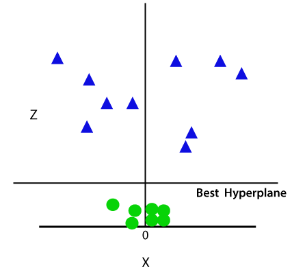
So now, SVM will divide the datasets into classes in the following way. Consider the below image:
Since we are in 3-d Space, hence it is looking like a plane parallel to the x-axis. If we convert it in 2d space with z=1, then it will become as:
Hence we get a circumference of radius 1 in case of non-linear data.
Important Concepts in SVM
The above explanation regarding the functioning of the support vector machines gives rise to a few phenomena and concepts that must be understood before we start applying SVM in the machine learning setup.
- Support Vectors
Support vectors are those data points on whose basis the margins are calculated and maximized. The number of support vectors or the strength of their influence is one of the hyper-parameters to tune discussed below.
- Hard Margin
This is an important concept in the understanding of SVM classification and support vector machines in general. Hard Margin refers to that kind of decision boundary that makes sure that all the data points are classified correctly. While this leads to the SVM classifier not causing any error, it can also cause the margins to shrink thus making the whole purpose of running an SVM algorithm futile.
- Soft Margin
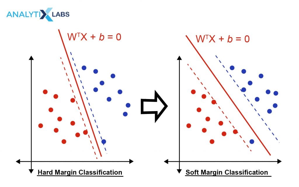
As mentioned above, a regularization parameter is also added to the loss function in the SVM classification algorithm. This combination of the loss function with the regularization parameter allows the user to maximize the margins at the cost of misclassification. However, this classification needs to be kept in check, which gives birth to another hyper-parameter that needs to be tuned.
- Different Kernels
The use of kernels is why the Support Vector Machine algorithm is such a powerful machine learning algorithm. As evident from all the discussion so far, the SVM algorithm comes up with a linear hyper-plane. However, there are circumstances when the problem is non-linear, and a linear classifier will fail. This is where the concept of kernel transformation comes in handy. By performing kernel transformation, a low dimensional space is converted into a high dimensional space where a linear hyper-plane can easily classify the data points, thus making SVM a de facto non-linear classifier. Different types of kernels help in solving different linear and non-linear problems. Selecting these kernels becomes another hyper-parameter to deal with and tune appropriately.
 Start Coding Today! Enroll Now with Easy EMI Options.

Equip yourself with in-demand skills to land top-tier roles in the data-driven world.
Start Learning Now with EMI OptionsAdvantages & Disadvantages of SVM
Each machine learning algorithm has its own set of advantages and disadvantages that makes it unique. The SVM algorithm is no different, and its pros and cons also need to be taken into account before this algorithm is considered for developing a predictive model.
Advantages
- It is one of the most accurate machine learning algorithms.
- It is a dynamic algorithm and can solve a range of problems, including linear and non-linear problems, binary, binomial, and multi-class classification problems, along with regression problems.
- SVM uses the concept of margins and tries to maximize the differentiation between two classes; it reduces the chances of model overfitting, making the model highly stable.
- Because of the availability of kernels and the very fundamentals on which SVM is built, it can easily work when the data is in high dimensions and is accurate in high dimensions to the degree that it can compete with algorithms such as Naïve Bayes that specializes in dealing with classification problems of very high dimensions.
- SVM is known for its computation speed and memory management. It uses less memory, especially when compared to machine vs deep learning algorithms with whom SVM often competes and sometimes even outperforms to this day.
Disadvantages
- While SVM is fast and can work in high dimensions, it still fails in front of Naïve Bayes, providing faster predictions in high dimensions. Also, it takes a relatively long time during the training phase. Many a time before SVM modeling you may also have use dimension reduction techniques like Factor Analysis or PCA (Principal Component Analysis)
- Like some other machine learning algorithms, which are often highly sensitive towards some of their hyper-parameters, SVM’s performance is also highly dependent upon the kernel chosen by the user.
- Compared to other linear algorithms such as Linear Regression, SVM is not highly interpretable, especially when using kernels that make SVM non-linear. Thus, it isn’t easy to assess how the independent variables affect the target variable.
- Lastly, a good amount of computational capability might be required (especially when dealing with a huge dataset) in tuning the hyper-parameters such as the value of cost and gamma.
With all its advantages and disadvantages, SVM is a widely implemented algorithm. Support vector machine examples include its implementation in image recognition, such as handwriting recognition and image classification. Other implementation areas include anomaly detection, intrusion detection, text classification, time series analysis, and application areas where deep learning algorithms such as artificial neural networks are used.
Enroll in our certificate program in data science and Machine learning
Conclusion
In this blog , we have learned about SVM Algorithm In Machine Learning, SVM algorithm steps and SVM algorithm formula. Any Data Scientist involved in developing predictive models must have a decent knowledge of the working of Support Vector Machine. SVM is easy to understand and even implement as the majority of the tools provide a simple mechanism to implement it and create predictive models using it. SVM is a sophisticated algorithm that can act as a linear and non-linear algorithm through kernels. As far as the application areas are concerned, there is no scarcity of domains and situations where SVM can be used. Being able to deal with high dimensional spaces, it can even be used in text classification.


