

Table of Contents
The pivot table is one of Microsoft Excel’s most powerful and daunting functions. You can use pivot tables to organize and summarize huge data sets. But, they are also known for being difficult.
You will understand the principles of pivot tables once you have finished reading this essay. You’ll be aware of their internal workings. Also, you’ll discover how to analyze your business data.
This article is for you if you have never made a pivot table or if you can but it seems magical to you.
Looking for a Data science and Machine learning Career? Explore Here!!
What is a Pivot Table?
A pivot table is a summary of your data presented in the form of a chart that allows you to report on and examine patterns depending on your data. With extensive rows or columns of information that you need to track sums of and quickly compare to one another, pivot tables are especially helpful.
To put it another way, pivot tables interpret the apparently infinite chaos of statistics on your screen. And more particularly, it enables you aggregate your data in multiple ways so you can draw beneficial conclusions more readily.
The “pivot” in a pivot table refers to the ability to spin or pivot the data within the table to see it from various angles. To be clear, when you perform a pivot, you are not increasing, decreasing, or otherwise altering your data. Instead, you are merely rearranging the data to make useful information more visible.
What are the uses of Pivot Tables in Excel?
1: Which of the following algorithms is most suitable for classification tasks?
The purpose of pivot tables is to provide simple methods for quickly summarizing vast volumes of data. They can be applied to more effectively comprehend, present, and thoroughly evaluate numerical data.
With this knowledge, you may assist in identifying and responding to unexpected inquiries regarding the data.
Comparing Sales Totals of Different Products
Consider that you have a worksheet with information on the monthly sales of three distinct products: product 1, product 2, and product 3. Find out which of the three has been bringing in the most money.
One approach would be to scan the spreadsheet and, each time product 1 appears, manually add the appropriate sales figure to a running total. Once you have totals for each product, you can repeat the process for products 2 and 3. Simple as pie, right?
Consider your monthly sales worksheet to have tens of thousands of rows. The amount of time it would take to manually sort through all the essential data is immeasurable.
With the help of pivot tables, you can quickly and easily total up all of the sales data for products 1, 2, and 3 and determine their individual amounts.
Showing Product Sales as Percentages of Total Sales
When built, pivot tables automatically display the sums for each row or column. Nevertheless, that is not the only figure you may generate automatically.
Consider creating a pivot table from data that you entered into an Excel sheet as quarterly sales figures for three different products. The pivot table calculates the quarterly sales for each product and displays three totals at the bottom of each column.
What if, however, you were looking for the proportion of overall business sales that these items’ sales made up as opposed to just their individual sales totals?
With a pivot table, you may customize each column to show you the percentage of all three column totals rather than simply the column total.
Let’s assume that sales of three products totaled $200,000. If you want to say that the first product contributed 22.5% of the business sales rather than that it brought in $45,000, you can update a pivot table.
Simply right-click the cell containing the sales total and choose Display Values As >% of Grand Total to display product sales in a pivot table as percentages of overall sales.
Combining Duplicate Data
In this case, you recently finished redesigning your blog and have to replace numerous URLs. The “view” metrics for individual posts were split across two separate URLs since your blog reporting software didn’t handle the transition correctly.
You now have two copies of each individual blog post in your spreadsheet. You must add the view totals for each of these duplicates in order to obtain accurate data.
You can use a pivot table to summarize your data by blog post title rather than having to manually find and combine all the metrics from the duplicates.
Suddenly, an automated aggregation of the view metrics from those duplicate posts will take place.
Getting an Employee Headcount for Separate Departments
Pivot tables can in handy for automatically calculating things that are difficult to locate in a straightforward Excel table. One of them is counting rows that share a characteristic.
Let’s imagine, for instance, that you have an Excel document with a list of your employees. The names of the employees’ relevant departments are shown next to their names. This information can be used to build a pivot table that displays the names of all the departments and their respective staff counts.
The automated features of the pivot table effectively take away your need to manually sort the Excel sheet by department name and count each entry.
Adding Default Values to Empty Cells
Not all datasets that you enter into Excel will fill up all of the cells. It’s possible that you have a large number of blank cells that appear confused or require more explanation while you’re waiting for new data to arrive.
This is where pivot tables come in.
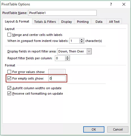
A pivot table can be readily customized to fill blank cells with a default value, such as $0 or TBD (for “to be determined”). When numerous persons are studying the same sheet, being able to easily tag these cells is a useful feature for huge data tables.
Right-click your pivot table and select PivotTable Options to automatically format the empty cells.
Check the box next to “Empty Cells As” in the resulting window, then type the text you want to appear when a cell is empty.
🚀 Start Coding Today! Enroll Now with Easy EMI Options. 💳✨
Equip yourself with in-demand skills to land top-tier roles in the data-driven world.
Start Learning Now with EMI OptionsHow to make a Pivot Table in Excel
A Pivot Table is thought to be time-consuming and labor-intensive by many individuals. Nevertheless, this is untrue! The technology has been improved by Microsoft over many years, and the summary reports in the most recent Excel versions are both extraordinarily quick and user-friendly. In reality, creating your own summary table only takes a few minutes. And this is how:
1. Organize your source data
Organize your data into rows and columns before generating a summary report, and then export your data range as an Excel Table. To do this, pick all of the data, then click Table on the Insert tab.
Your data range becomes “dynamic” when you use an Excel Table as the source data, which is a really pleasant bonus. In this case, the term “dynamic range” refers to a table that automatically grows and contracts as items are added or removed, so you won’t have to worry about your pivot table not having the most recent data.
Tips:
- Give your columns interesting, distinctive titles; they will later serve as the field names.
- Ensure that your source table has no subtotals, blank rows or columns, or any empty spaces.
- You can give your source table a name to make it simpler to maintain by selecting the Design tab and entering the name in the Table Name box in the worksheet’s top right corner.
2. Create a Pivot Table
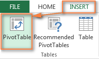
Go to the Insert tab > Tables group > PivotTable after selecting any cell in the source data table.
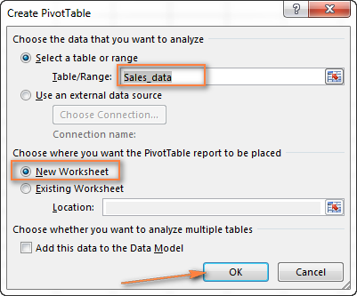
The Create PivotTable window will open as a result. Check to see that the appropriate table or cell range is highlighted in the Table/Range field. Next, decide where you want your Excel pivot table to be located:
- A table will be started in a new worksheet at cell A1 if you choose New Worksheet.
- When you choose an existing worksheet, your table will be inserted at the chosen spot in the worksheet. Click the Collapse Dialog button
 in the Location box. To place your table, select the first cell using the Collapse Dialog button.
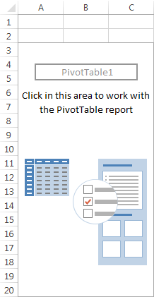
After you click OK, a blank Pivot Table is created at the target place, similar to this.
Tips:
- Most of the time, it makes sensible to include a pivot table in a separate worksheet; beginners are strongly advised to do this.
- When generating a pivot table from data in another worksheet or workbook, use the notation [workbook name] to include the names of the worksheet and workbook. for instance, [Book1] sheet name!range .xlsx] Sheet1!$A$1:$E$20. As an alternative, press the Collapse Dialog button. Use the mouse to pick a table or range of cells in another worksheet by clicking the Collapse Dialog button.
- A pivot table and pivot chart could be made at the same time. With Excel 2013 and later, select the Insert tab > Charts group, click the arrow next to the PivotChart button, and then select PivotChart & PivoTable to accomplish this. Click the arrow next to PivotTable in XLS 2010 and 2007 before selecting PivotChart.
Computer Keyboard – Parts, Functions, Quiz
3. Arrange the layout of your Pivot Table report
PivotTable Field List refers to the place where you deal with the fields in your summary report. It is divided into the header and body sections and is situated in the worksheet’s right-hand corner:
- The names of the fields that you can include in your table are listed in the Field Section. The names of the fields match the names of the columns in your source table.
- The Report Filter area, Column Labels area, Row Labels area, and Values area are all located in the Layout Section. The fields of your table can be rearranged and arranged here.
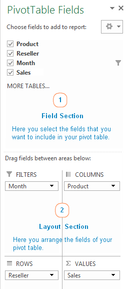
As you make changes to the PivotTable Field List, your table is updated right away.
How to add a field to Pivot Table
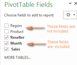
Choose the checkbox next to the field name in the Field section to add the field to the Layout section.
By default, Microsoft Excel includes the following fields to the Layout section:
- There are now non-numerical fields in the Row Labels section;
- The Values area now includes additional numerical fields;
- Date and time hierarchies from Online Analytical Processing (OLAP) are added to the Column Labels section.
How to remove a field from a Pivot Table
You have two options for deleting a specific field:
- In the PivotTable pane’s Field section, uncheck the box next to the field’s name.
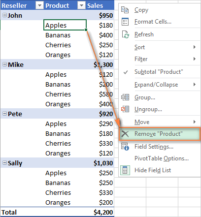
- Choose “Remove Field Name” from the context menu when you right-click on the field in your pivot table.
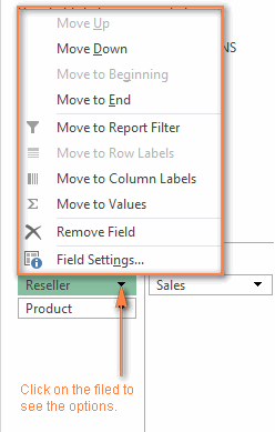
How to arrange Pivot Table fields
There are three ways you can arrange the fields in the Layout section:
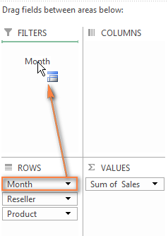
- Using the mouse, move fields among the four sections of the Layout section. The field can also be moved by clicking and holding the field name in the Field section while dragging it to a different location in the Layout section. This will shift the field from its present location in the Layout section to the new location.
- In the Field section, right-click the field name, then choose the location where you wish to add it:
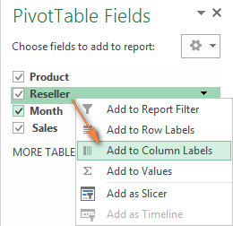
- To pick a field, click on it in the Layout section. Also, this will show the choices that are accessible for that specific field.
4. Choose the function for the Values field (optional)
If you put a numeric value field in the Values section of the Field List, Microsoft Excel will automatically apply the Sum function. The Count function is used when you enter text, date, Boolean, or other non-numeric data or empty values in the Values field.
But, if you like, you can select an alternative summary function. Choose the desired summary function by selecting Summarize Values By from the context menu when using Excel 2013 or later.
The Summarize Values By option is also included in Excel 2010 and before on the ribbon, under the Calculations group of the Options tab.
An illustration of a pivot table using the average function is provided below:
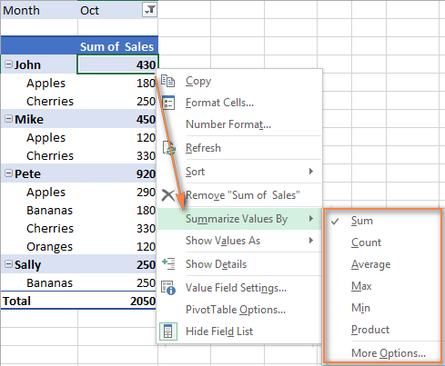
The names of the functions are generally self-explanatory:
- Sum – calculates the sum of the values.
- Count – counts the number of non-empty values (works as the COUNTA function).
- Average – calculates the average of the values.
- Max – finds the largest value.
- Min – finds the smallest value.
- Product – calculates the product of the values.
Click Summarize Values By > More Options to get more specific functions. The complete list of available summary functions and their in-depth descriptions may be found here.
Looking for a Data science and Machine learning Career? Explore Here!!
5. Show different calculations in value fields (optional)
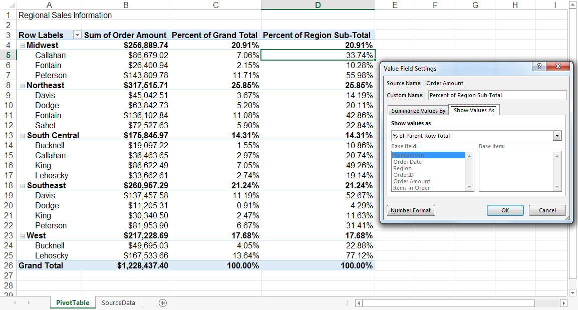
Another helpful feature offered by Excel pivot tables is the ability to present values in various ways, such as showing totals as percentages or ranking values from smallest to largest and vice versa.
In Excel 2013 and later, you may use this function named Display Values As by right-clicking the field in the table. This option is also available in the Calculations group of the Settings tab in Excel 2010 and before.
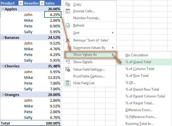
Tip:
Values of the Show If you add the same field more than once and display, for instance, total sales and sales as a percent of total at the same time, this functionality might prove to be extremely helpful. View a sample of one of these tables.
This is how Pivot Tables are made in Excel. Now it’s up to you to play about with the fields a little to find the arrangement that works best for your set of data.
Working with Pivot Table Field List
The major tool you employ to set up your summary table exactly how you desire is the Pivot Table pane, which is also known as the PivotTable Field List. You might wish to adjust the pane to your preferences to make working with the fields more comfortable.
Changing the Field List view
Click the Tools button and select your preferred layout to alter how the sections are shown in the Field List.
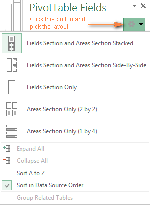
By dragging the bar (splitter) that divides the pane from the worksheet, you can also resize it horizontally.
Closing and opening the Pivot Table pane
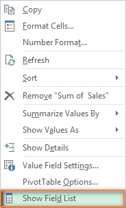
Simply click the Close button (X) in the top right corner of the pane to close the PivotTableField List. It is not as easy to make it appear once more.
Right-click anywhere in the table, then choose Show Field List from the context menu to bring up the Field List once more.
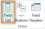
Moreover, you can use the Field List button on the Ribbon, which is found in the Display group of the Analyze / Options tab.
Using Recommended Pivot Tables
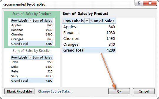
As you’ve just seen, it’s simple to create a pivot table in Excel. Modern Excel versions go one step further, though, and allow you to create a report that’s specifically tailored to your source data automatically. You only need to make 4 mouse clicks:
- Click any cell in the table or cell range that is your source.
- Then select Suggested PivotTables from the Insert tab. Based on your data, Microsoft Excel will immediately present a few layouts.
- To view a layout’s preview in the Suggested PivotTables dialog box, click a layout.
- Click the OK button when you are satisfied with the preview to add a pivot table to a new worksheet.
How to use Pivot Table in Excel
Now that you are familiar with the basics, you may explore the groups and choices offered by the PivotTable Tools in Excel 2013 and later by navigating to the Analyze and Design tabs (Options and Design tabs in Excel 2010 and 2007). You can access these tabs by clicking anywhere in your table.
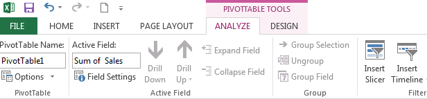
Right-clicking on an element gives you access to the features and settings that are applicable to that element.
Ready to take your data science skills to the next level? Sign up for a free demo today!
How to refresh a Pivot Table in Excel
Although a Pivot Table report is linked to your source data, you might be stunned to learn that Excel does not immediately refresh it. Any updates to the data can be obtained manually, or they can be automatically updated when you access the spreadsheet.
Refresh the Pivot Table data manually
- In your table, click anywhere.
- Click the Refresh button or press ALT+F5 in the Data group of the Analyze tab (the Options tab in previous iterations).
The table can also be selected by right-clicking it and selecting Refresh from the context menu.
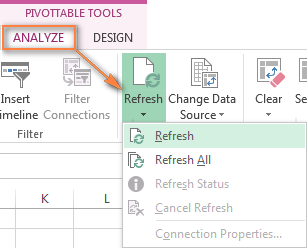
Click the arrow next to the Refresh button to open the menu, then select Refresh All to update every Pivot Table in your workbook.
You can check the status after starting a refresh or, if you’ve changed your mind, stop it. Simply click the arrow next to the Refresh button, and then select Refresh Status or Cancel Refresh.
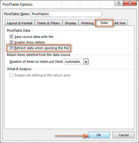
Refreshing a Pivot Table automatically when opening the workbook
- Click Options > Options under the PivotTable group on the Analyze / Options tab.
- Choose the Refresh data when opening the file check box on the Data tab of the PivotTable Settings dialog box.
How to design and improve Pivot Table
If you wish to perform powerful data analysis, you might want to further enhance your Pivot Table after you have generated it using your source data.
Go to the Design tab, where you will find a ton of pre-defined styles, to enhance the table’s appearance. To build your own style, select “New PivotTable Style…” from the menu that appears after clicking the More button in the PivotTable Styles gallery.
In Excel 2013 and later, click on the field you want to change, then select the Field Settings button on the Analyze tab (Options tab in Excel 2010 and 2007). As an alternative, you can use the context menu that appears when you right-click a field to select Field Options.
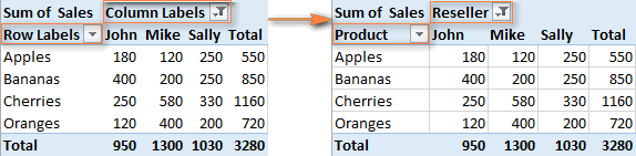
How to get rid of “Row Labels” and “Column Labels” headings
Excel uses the Compact layout by default when you create a Pivot Table. The table headings in this style are “Row Labels” and “Column Labels”. I agree that these titles aren’t particularly informative, especially for beginners.
By switching from the Compact layout to Outline or Tabular, you may quickly get rid of these ludicrous headings. To do this, select Show in Outline Form or Show in Tabular Form from the Report Layout dropdown menu on the Design ribbon tab.
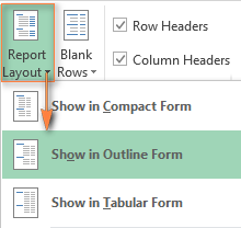
This makes much more sense because it will show the real field names, as you can see in the table on the right.
🚀 Start Coding Today! Enroll Now with Easy EMI Options. 💳✨
Equip yourself with in-demand skills to land top-tier roles in the data-driven world.
Start Learning Now with EMI OptionsPivot Table examples
The screenshots below show a few different Pivot Table layouts that might be used with the same source data and could guide you in the right direction.
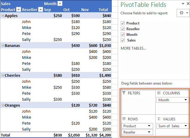
Pivot Table example 1: Two-dimensional table
- No Filter
- Rows: Product, Reseller
- Columns: Months
- Values: Sales
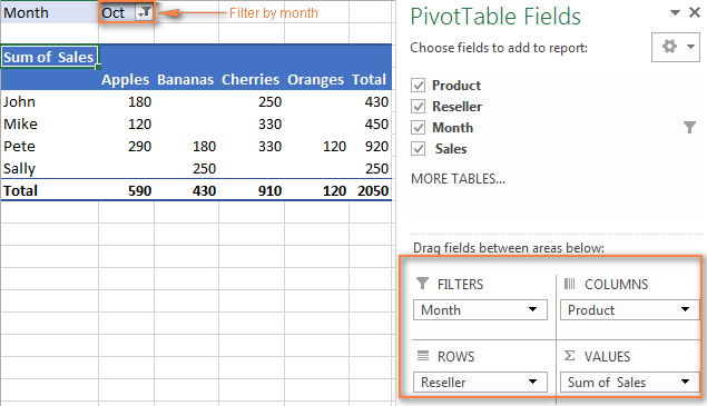
Pivot Table example 2: Three-dimensional table
- Filter: Month
- Rows: Reseller
- Columns: Product
- Values: Sales
This Pivot Table lets you filter the report by month.
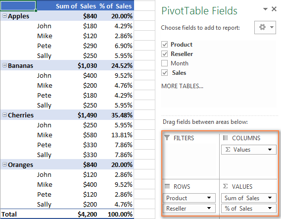
Pivot Table example 3: One field is displayed twice – as total and % of total
- No Filter
- Rows: Product, Reseller
- Values: SUM of Sales, % of Sales
The overall sales and the sales as a percentage of the total are both shown in this summary report.
Looking for a Data science and Machine learning Career? Explore Here!!
| Related Links | |
| Pivot Table in Excel | Top Excel Interview Questions |
| Basic Excel Formulas and Functions | Keyboard Shortcuts in Excel |
| Advanced Excel Formulas | Six Sigma |


