Microsoft Excel, a spreadsheet software that lets you manage and analyze data. If you are a beginner or a pro, Excel offers a wide variety of features that may assist you with data analysis and documentation. If your job requires you to manage data, you should be familiar with Microsoft Excel Formulas and their functions.
So in this article we are discussing the most advanced Excel formulas that may be useful for those who are looking job in data management field.
Looking for a Data science and Machine learning Career? Explore Here!!
Top 10 Advanced Excel formulas with examples in Excel sheet Free Download
1. IF combined with AND / OR
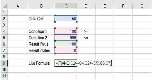
Formula: =IF(AND(C2>=C4,C2<=C5),C6,C7)
Combining IF with the AND or the OR function can be a great way to keep formulas easier to audit and easier for other users to understand.
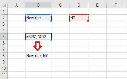
2. CONCATENATE
Formula: =A1&” more text”
This is a very powerful tool for financial analysts performing financial modeling.
3. SUMIF and COUNTIF
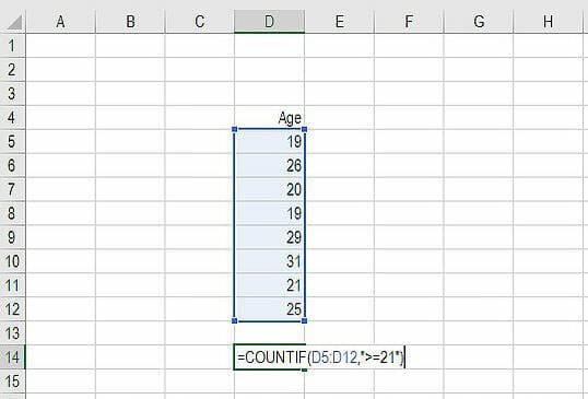
Formula: =COUNTIF(D5:D12,”>=21″)
These two advanced formulas are great uses of conditional functions. SUMIF adds all cells that meet certain criteria, and COUNTIF counts all cells that meet certain criteria.
Ready to take your data science skills to the next level? Sign up for a free demo today!
4. PMT and IPMT
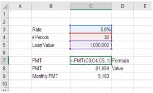
Formula: =PMT(interest rate, # of periods, present value)
The PMT formula gives you the value of equal payments over the life of a loan. You can use it in conjunction with IPMT (which tells you the interest payments for the same type of loan), then separate principal and interest payments.
5. XNPV and XIRR
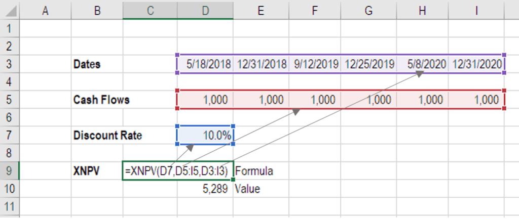
Formula: =XNPV(discount rate, cash flows, dates)
This formula allows you to apply specific dates to each individual cash flow that’s being discounted. The problem with Excel’s basic NPV and IRR formulas is that they assume the time periods between cash flow are equal. Sometimes, as an analyst, you’ll have to face the situations where cash flows are not timed evenly, and this formula will help you to fix it.
6. CHOOSE
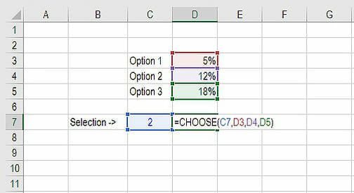
Formula: =CHOOSE(choice, option1, option2, option3)
This formula allows you to pick between a specific number of options, and return the “choice” that you’ve selected.
7. OFFSET combined with SUM or AVERAGE
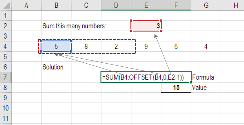
Formula: =SUM(B4:OFFSET(B4,0,E2-1))
To run this formula, we substitute the ending reference cell of the SUM function with the OFFSET function. This makes the formula dynamic and the cell referenced as E2 is where you can tell Excel how many consecutive cells you want to add up.
8. INDEX MATCH
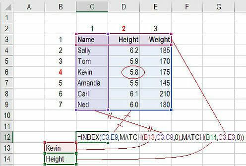
Formula: =INDEX(C3:E9,MATCH(B13,C3:C9,0),MATCH(B14,C3:E3,0))
This is a powerful combination of Excel formulas that will take your financial analysis and financial modeling to the next level.
INDEX returns the value of a cell in a table based on the column and row number.
MATCH returns the position of a cell in a row or column.
Looking for a Data Science Career? Explore Here!
9. LEN and TRIM
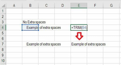
Formulas: =LEN(text) and =TRIM(text)
These formulas are very useful for financial analysts who are dealing with large amount of data. Unfortunately, the data we get is not always perfectly organized and sometimes, there can be issues like extra spaces at the beginning or end of cells.
The LEN formula returns a given text string as the number of characters, which is useful when you want to count how many characters there are in some text.
The TRIM formula cleans up the extra spaces in the Excel data.
10. CELL, LEFT, MID and RIGHT
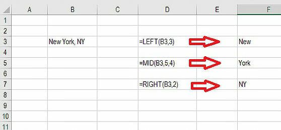
These excel functions can be combined to create advanced and complex formulas to use.
The CELL function can return a variety of information about the contents of a cell (such as its name, location, row, column, and more).
The LEFT function can return text from the beginning of a cell (left to right).
The MID returns text from any start point of the cell (left to right).
The RIGHT returns text from the end of the cell (right to left).
Some Basic Excel Formulas
- SUM: Calculates the sum of a range of cells. Example: =SUM(A1:A10)
- AVERAGE: Calculates the average of a range of cells. Example: =AVERAGE(A1:A10)
- MAX: Returns the maximum value in a range of cells. Example: =MAX(A1:A10)
- MIN: Returns the minimum value in a range of cells. Example: =MIN(A1:A10)
- COUNT: Counts the number of cells in a range that contain a value. Example: =COUNT(A1:A10)
- IF: Returns one value if a condition is true and another value if it is false. Example: =IF(A1>10, “Greater than 10”, “Less than or equal to 10”)
- VLOOKUP: Searches for a value in the first column of a table and returns a corresponding value in the same row from another column. Example: =VLOOKUP(A1, B1:C10, 2, FALSE)
- CONCATENATE: Combines two or more text strings into one. Example: =CONCATENATE(“John”, ” “, “Doe”)
- LEFT: Returns a specified number of characters from the beginning of a text string. Example: =LEFT(A1, 5)
- RIGHT: Returns a specified number of characters from the end of a text string. Example: =RIGHT(A1, 5)
| Related Links | |
| Pivot Table in Excel | Top Excel Interview Questions |
| Basic Excel Formulas and Functions | Keyboard Shortcuts in Excel |
| Advanced Excel Formulas | Six Sigma |


